User guide
1 Overview
The application is online here and consists of four separate pages or “tabs”, which are selected from the left sidebar:
Forside displays a welcome message and a link to this documentation.
Innsjømodellering allows users to:
- Explore column test results for lime products in the application’s database.
- Specify lake characteristics and liming parameters, which are then used to simulate changes in lake water chemistry (calcium-equivalent concentration and pH).
Omregningsfaktorer shows plots comparing the modelled effectiveness of different lime products for a range of lake characteristics (mean depths and water residence times). Generating these plots involves running the model many times, so for efficiency they are pre-computed and presented here for reference.
Last opp kolonnetestdata allows users to upload their own column test data (i.e. for lime products not already in the database). Users may download and fill-in an Excel template, which can then be uploaded using the
Browse filesbutton. The app will display plots of instantaneous dissolution and overdosing factors based on the data provided.
2 Lake modelling
The Innsjømodellering tab is the main page of the application and is divided into four sections: Liming products, Lake characteristics, Liming parameters and Model results. Under each heading, you will find expandable Help boxes providing tips for how to use the app.
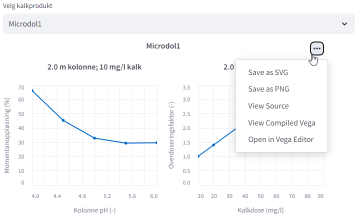
2.1 Liming products
Select your product of interest using the drop-down list labelled Choose liming product. The app will display plots of instantaneous dissolution and overdosing factors based on the latest column test data in the database. Click the ellipsis button ([...]) that appears near the top-right of the plot area to export the plots in PNG or SVG format (Figure 1).
See the Column tests page for a detailed description of the laboratory tests on which these plots are based.
2.2 Lake characteristics
Use the input boxes to enter data for you lake of interest.
Surface area and mean depth are used to estimate lake volume. The ratio of lake volume to mean annual discharge volume is the water residence time (in years), which is the length of time, on average, that water spends circulating in the lake. The initial pH of the lake and the inflow pH are used to define the water chemistry at the start of the simulation. For lakes that are unlimed, or which have not been limed for a long time, it can be assumed that initial pH and inflow pH are equal, whereas recently limed lakes will typically have initial pH > inflow pH. If no additional lime is added, the pH of the model lake will tend towards the inflow pH at a rate determined by the water residence time (lakes with shorter residence times reach the inflow pH faster). The Total Organic Carbon (TOC) concentration in the lake is also important, as the presence of organic acids means that more lime will be needed to achieve a given change in pH (see Lake moodelling for details).
Users must also specify a Flow profile, which determines the idealised monthly flow regime used by the model (see the plot here for details). Three choices are available:
- None. Monthly flows are constant throughout the year.
- Fjell. The profile is characterised by high springtime flows (associated with snow-melting), a wet autumn, and low flows during the winter. Suitable for simulating upland lakes with significant snow accumulation.
- Kyst. The profile is characterised by dry summers with wet autumns and winters. Suitable for lowland lakes with little snow accumulation.
If Flow profile is None, the flow rate is determined from the lake volume and water residence time. For Fjell and Kyst, monthly values are scaled to match the chosen pattern, but the mean annual flow rate remains the same (i.e. consistent with the specified lake volume and water residence time).
2.3 Liming parameters
Use the input boxes to define the liming schedule. The lime dose is the amount of product added divided by the volume of water limed. In cases where lime is only spread over part of a lake’s surface, use Proportion of lake surface area limed to specify the extent of liming. If this value is less than one, it is assumed that the lake depth profile is such that liming e.g. half of the surface area is equivalent to liming half of the lake volume.
The model assumes that the lake eventually becomes well-mixed, regardless of the areal extent of liming. Adding 10 mg/l of lime product over the whole lake is therefore similar to adding 20 mg/l over 50% of the surface area. However, in the latter case, overdosing effects will modify the instantaneous dissolution, meaning that slightly less lime will dissolve immediately and more will sink to the lake bottom (and potentially dissolve later). See the Lake modelling page for details.
Application method can be either Wet or Dry, where Wet corresponds to adding lime as a slurry (e.g. from a boat) and Dry corresponds to adding raw material directly without any pre-mixing (e.g. from a helicopter). Dry lime dissolves in lake water more slowly than slurry. If Dry is selected, instantaneous dissolution values from the column tests are adjusted downwards to account for this.
Application month is the month of the year in which liming takes place and Number of months to simulate determines the length of time series generated. If Flow profile is set to None (Section 2.2), Application month will have no effect, because flows remain constant throughout the year. However, for the Fjell and Kyst profiles application month can be important - especially for upland lakes with short residence times, where water is cycled quickly during spring snow-melt episodes.
2.4 Model results
Changing values in any of the input boxes will automatically trigger an update of the model results. While this happens, a RUNNING message will be displayed at the top-right of the screen.
When the model run is finished, the application will display idealised time series of Ca-equivalent concentration and pH for the number of months specified. Simulations are produced for all lime products in the database, making it easy to compare results for different products.
The plots are interactive - expand the Help section under the Model results heading for an overview of how to explore them.
Time series produced by the model are based on generalised/typical relationships that do not account for local factors (which may be important). Results indicate the expected response of a typical lake, but are not intended for detailed, site-specific assessments.
3 Omregningsfaktorer
Plots of “omregningsfaktorer” are a convenient way to compare the simulated effectiveness of different lime products in lakes with different characteristics. To generate the plots, initial conditions are defined for a broad range of lakes with varying mean depth and water residence time. The model is then run many times to identify how much of each lime product would be required to achieve a given pH target after some period of time (e.g. one year).
For each lime product, the amount of lime required (in tonnes) is compared to results for a standard “reference” product to give the omregningsfaktor. The reference used by this application is Standard Kalk Kat3. Values less than one indicate the product being tested is more effective than the standard, while values greater than one imply it is less effective (per unit mass).
In principle, these plots could be constructed manually using the Innsjømodellering page. However, the number of parameter combinations is large, so for efficiency they are pre-computed for all lime products in the database and presented on this page in summary form. Plots are generated for lakes with mean depths of 5, 10, 15 and 20 m, and curves shown for lakes with water residence times ranging from 0.3 to 2 years.
Differences between products on these plots reflect the different physical and chemical properties of the limes, as represented by the column test data.
4 Column tests
The Laste opp kolonnetestdata page can be used to create plots of instantaneous dissolution and overdosing factors based on user-supplied column test data.
You can explore column test results for lime products that are already in the application’s database from the Innsjømodellering tab.
To create plots based on your own data, first download a blank copy of the Excel input template from here. Fill-in the template and save the changes on your local machine, then upload the completed Excel file to the web application by clicking the Browse files button in the left sidebar. The app will display plots of instantaneous dissolution and overdosing factors based on the data you provide.
Data uploaded via the Laste opp kolonnetestdata tab is not immediately added to the application database. If you want to add a new product to the application (or update information for an existing one), first fill-in the Excel template and check the plots look reasonable. You can then send the completed template to NIVA for inclusion in the product database.