Lake modelling
The calculations performed by the application and described on this page are a subset of those implemented by the original TPKALK application developed by NIVA during the 1990s.
1 Background
1.1 Types of liming material
Lime products used for catchment management are usually a mixture of calcium carbonate (calcite, \(CaCO_3\)) and magnesium carbonate (\(MgCO_3\)). Rocks composed primarily of \(CaCO_3\) are commonly called limestones and chalks, whereas carbonate rocks with significant proportions of magnesium are called dolomites (> 10% Mg) or magnesian limestones (2 to 10% Mg).
Lime manufacturers will typically specify the proportion of calcium and magnesium carbonate in their products. For example, Microdol5 is reported as being 53.7% \(CaCO_3\) and 44.4% \(MgCO_3\) by mass (with 1.9% other impurities).
Magnesium carbonate has a higher proportion of carbonate by mass (and therefore a greater acid neutralising capacity; ANC) than calcium carbonate: 1 g of magnesium carbonate will neutralise as much acid as 1.19 g of calcium carbonate. When comparing limes with different compositions, it is therefore necessary to multiply the magnesium carbonate proportion by a factor of 1.19. This gives a neutralising value (NV), estimated as the sum of calcium carbonate equivalents (e.g. Table 1). The NV is best determined by titration according to EN-12945. It may also be estimated from Ca and Mg element analyses, but in some cases these elements may be fixed to minerals other than carbonates with little or no neutralising capacity.
| Product | CaCO3 (%) | MgCO3 (%) | MgCO3 (CaCO3-ekv; %) | NV (sum of CaCO3-ekv; %) |
|---|---|---|---|---|
| Microdol5 | 53.7 | 44.4 | 52.8 | 106.5 |
| VK3 | 99.0 | 1.0 | 1.2 | 100.2 |
The NV is usually specified in percent: pure calcium carbonate has a NV of 100 %; pure magnesium carbonate has a NV of 119 %; and typical dolomite products have NVs that are somewhere in between. For the same mass, products with a higher NV will be more effective at increasing pH, as long as all the lime dissolves. In practice, different limes exhibit different dissolution rates, which must also be accounted for (Section 1.2).
1.2 Lime solubility
Several factors affect the dissolution rate of lime material added to a waterbody. These include:
Physical and chemical properties of the liming material (crystal structure etc.).
Particle size (i.e. fineness) of the lime material. Smaller particles give a larger reaction surface and therefore dissolve faster.
Water pH. More acidic lakes react with the lime more vigorously.
Application method (for example from a boat versus from a helicopter).
Amount of lime added, usually called the dose. If large amounts of lime are added to a lake all at once, the overall effect on pH is less than might be achieved if smaller amounts were added more regularly. This is because, at high doses, pH and calcium concentration increase in the immediate vicinity of the lime particles, which then sink to the bottom without dissolving efficiently. It is also more likely that lime particles will clump together and sink more rapidly. This effect is called overdosing.
Most commercial lime products are fine enough to dissolve effectively. For a given application method and lake pH, the goal is therefore to identify which lime product to use (i.e. which physical and chemical properties to select) and in what dose (to minimise the number of applications necessary, without excessive waste due to overdosing).
Lime dissolution rates and the effects of overdosing are determined experimentally - see the column tests page for details.
2 Modelling procedure
The goal of the model is to simulate changes in lake pH due to liming with different products. It provides one part of the evidence base to decide which lime products to apply under different circumstances.
The model attempts to simulate a “typical” lake and results must therefore be considered as illustrative. Measured data from real lakes demonstrates that dose-response relationships are highly variable and may depend strongly on local factors. The model uses idealised empirical relationships based on Norwegian monitoring data and lab tests. It is not designed for detailed simulation of individual lakes.
2.1 Relationship between Ca-equivalents and pH
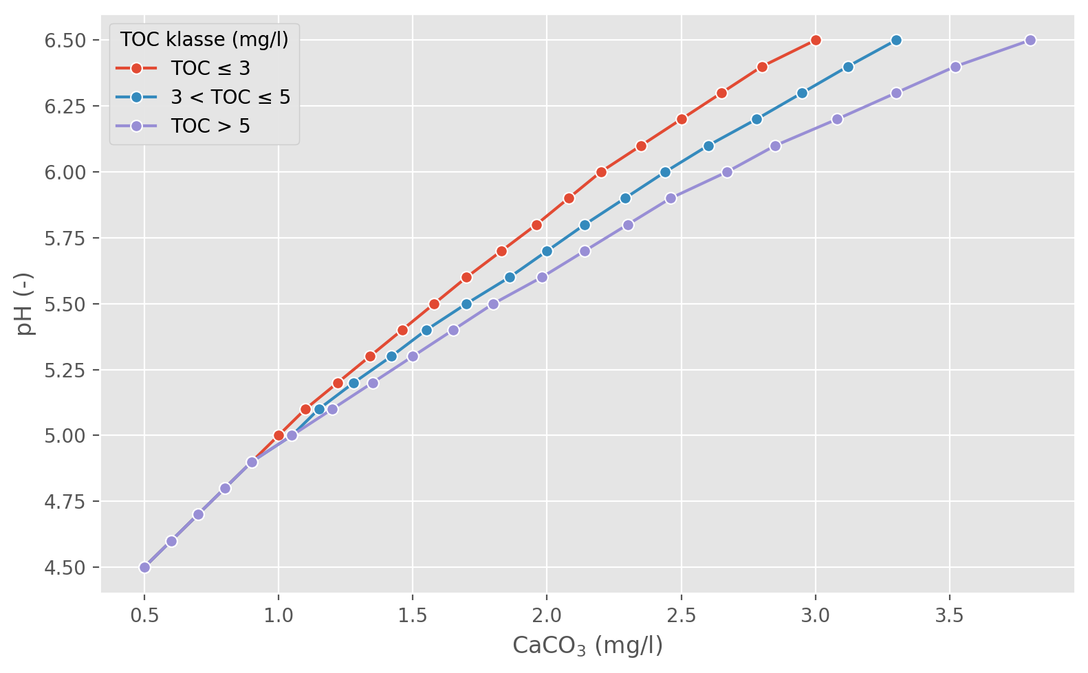
When we add liming material, the concentration of CaCO3 (and MgCO3, if relevant) in the lake increases, which leads to an increase in pH. Figure 1 shows relationships derived empirically by Atle Hindar relating changes in CaCO3-equivalents to changes in pH for lakes with different concentrations of Total Organic Carbon (TOC).
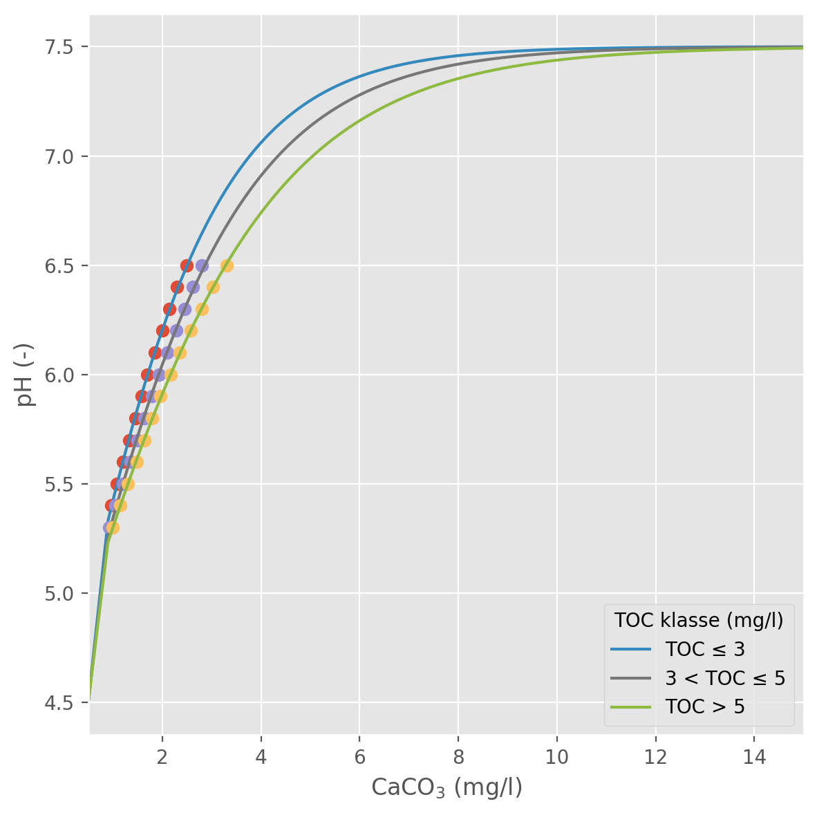
For a lake with a given initial pH and TOC concentration, the model uses sigmoid curves based on the empirical data (Figure 2) to lookup an idealised CaCO3 concentration representing the initial buffering capacity of the lake. The model then simulates changes in CaCO3-equivalent concentrations over time (relative to the initial concentration), and uses the curves to estimate corresponding changes in pH.
2.2 Mass balance model
The titration curves in Figure 2 transform the problem of modelling pH into one of modelling \(\Delta Ca\) (and \(\Delta Mg\) too, if relevant). When we add lime to a lake, some of it dissolves instantly, giving a sudden increase in pH, while the remainder sinks to the bottom and dissolves more slowly.
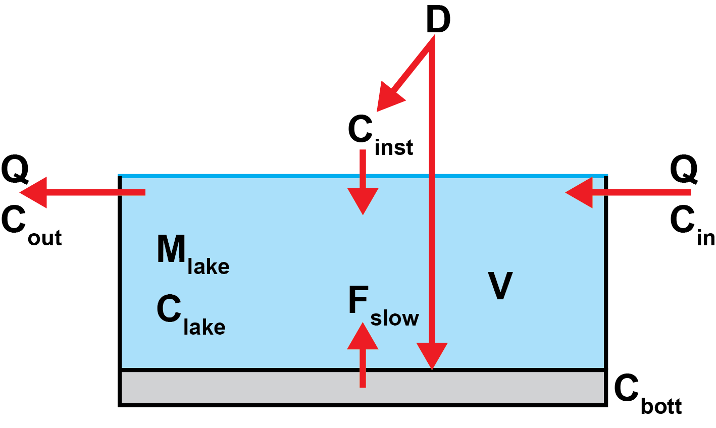
A mass balance “box model” (Figure 3) is used to provide an estimate of both the initial change in lake conditions due to liming and the subsequent evolution over time. For simplicity, only one set of calculations is shown (e.g. for calcium), but an identical set of calculations for magnesium are also performed in parallel, if relevant. The Mg-fraction is then converted to CaCO3-equivalents before making the link to changes in pH (Section 2.1). Taking calcium as an example, the symbols in Figure 3 are as follows:
- \(D\) is the dose of lime added (adjusted for Ca content i.e. the actual dose of Ca in mg/l).
- \(C_{inst}\) is the “immediate” increase in lake Ca concentration (in mg/l) due to instantaneous dissolution.
- \(C_{bott} = (D - C_{inst})\) is the amount of Ca (in mg/l) that sinks to the lake bottom and dissolves more slowly.
- \(F_{slow}\) is the rate at which concentration increases (in mg/l/month) due to dissolution of the bottom layer.
- \(C_{in}\) and \(C_{out}\) are the inflow and outflow concentrations of Ca, respectively (both in mg/l).
- \(V\) is the lake volume in litres. The lake is assumed to be in steady state i.e. \(V\) is constant.
- \(Q\) is the discharge in l/month. To satisfy the steady state assumption, the inflow discharge must equal the outflow discharge.
- \(M_{lake}\) is the mass of Ca dissolved in the lake water (in mg).
- \(C_{lake}\) is the Ca concentration in the lake, equal to \(\frac{M_{lake}}{V}\). The lake is assumed to be well mixed, such that the outflow concentration, \(C_{out}\), is equal to \(C_{lake}\).
Balancing the main sources and sinks of Ca to the lake gives
\[ \frac{dM_{lake}}{dt} = V \frac{dC_{lake}}{dt} = Q C_{in} - Q C_{lake} + V C_{inst} + V F_{slow} \tag{1}\]
or
\[ \frac{dC_{lake}}{dt} = \frac{Q C_{in} - Q C_{lake}}{V} + C_{inst} + F_{slow} \tag{2}\]
Lime that does not dissolve instantly sinks to the bottom of the lake and dissolves more slowly (\(C_{bott}\)). Dissolution of lake-bottom lime is modelled as a first-order reaction with initial rate coefficient \(K_0\). However, this rate coefficient is assumed to decay exponentially over time, based on the observation that lime accumulating in lake sediments becomes less “active” over time and therefore dissolves more slowly. The rate at which the reaction coefficient decays is controlled by the “activity coefficient”, \(\lambda\)
\[ K_t = K_0 e^{- \lambda t} \tag{3}\]
where \(K_t\) is the first order reaction coefficient at time \(t\).
The effective rate coefficient, \(K_t\), is further modified by a “rate factor”, \(R\), which reduces the dissolution rate as concentrations of dissolved CaCO3 in the lake become high. In particular, \(R\) forces \(K_t\) towards zero as dissolved concentrations approach saturation. This is done primarily to ensure the model’s output remains plausible even if users set extreme parameter values in the user interface; for most realistic choices of input parameters, lake concentrations will not approach saturation and the value of \(R\) will be close to 1.
\[ R = \frac{1}{1 + e^{10 (C_{lake} - C_{sat})}} \tag{4}\]
where \(C_{sat}\) is the saturation concentration of Ca in lake water (i.e. the maximum value permitted by the model).
\[ F_{slow} = - \frac{dC_{bott}}{dt} = C_{bott} K_t R \tag{5}\]
2.3 Estimating instantaneous dissolution
For the model to produce reasonable simulations, it is important to have an accurate estimate for the proportion of lime material that dissolves quickly (i.e. the instantaneous dissolution fraction, \(C_{inst}\)). Instantaneous dissolution can be measured in the laboratory using column tests, which tell us how much lime will typically dissolve in a column given a known initial pH and lime dose. However, before the column test data can be used for lake modelling, it is necessary to adjust for:
Spreading method. For dry spreading (e.g. by helicopter) the amount of lime material that dissolves immediately is typically 0.5 to 0.7 times the proportion predicted by column tests. No adjustment is required for wet spreading (e.g. from a boat).
Lake depth. Deeper lakes give the lime more time to dissolve as it sinks. In his PhD thesis, Sverdrup (1985) noted that, for CaCO3, the instantaneous dissolution is directly proportional to both \(H^+\) concentration and sinking depth
\[ D_{inst} \propto [H^+] \times d \tag{6}\]
It is therefore possible to generalise instantaneous dissolution estimates from fixed-depth column tests to lakes with different depths by considering compensating changes in pH. For example, the expected dissolution for lake of depth \(d\) and hydrogen ion concentration \(H^+\) is the same as for a lake with depth \(2d\) and hydrogen ion concentration \(0.5H^+\). Re-writing in terms of pH, the instantaneous dissolution for a lake of depth \(d_{lake}\) and initial pH \(X\) is assumed to be similar to the dissolution in a test column of depth \(d_{col}\) with pH \((X - a)\) where
\[ a = log(\frac{d_{lake}}{d_{col}}) \tag{7}\]
Note that Equation 7 applies to the CaCO3 fraction; for MgCO3, Sverdrup proposed the modification \((X - 0.5a)\) as a more appropriate depth correction.
2.4 Simulating a “standard lake”
The model defined above is capable of simulating how pH and Ca concentration (and Mg, if relevant) change over time for a single lake. The model requires the following inputs:
Lake volume (often provided as surface area and mean depth) and discharge, which together define the residence time. Note that this model assumes the volume is fixed, but discharge can vary over time, if desired.
Lake pH, inflow pH and TOC concentration.
The dose of liming material added and the proportion of Ca and Mg by mass in the lime. Overdosing factors are also relevant for higher doses.
Lake mean depth and Spreading method (i.e. “wet” or “dry”), both of which are used to adjust the instantaneous dissolution values from column tests (Equation 7).
The parameters \(K_0\) and \(\lambda\), which determine how fast lime on the lake bottom dissolves, and how long it remains “active”.
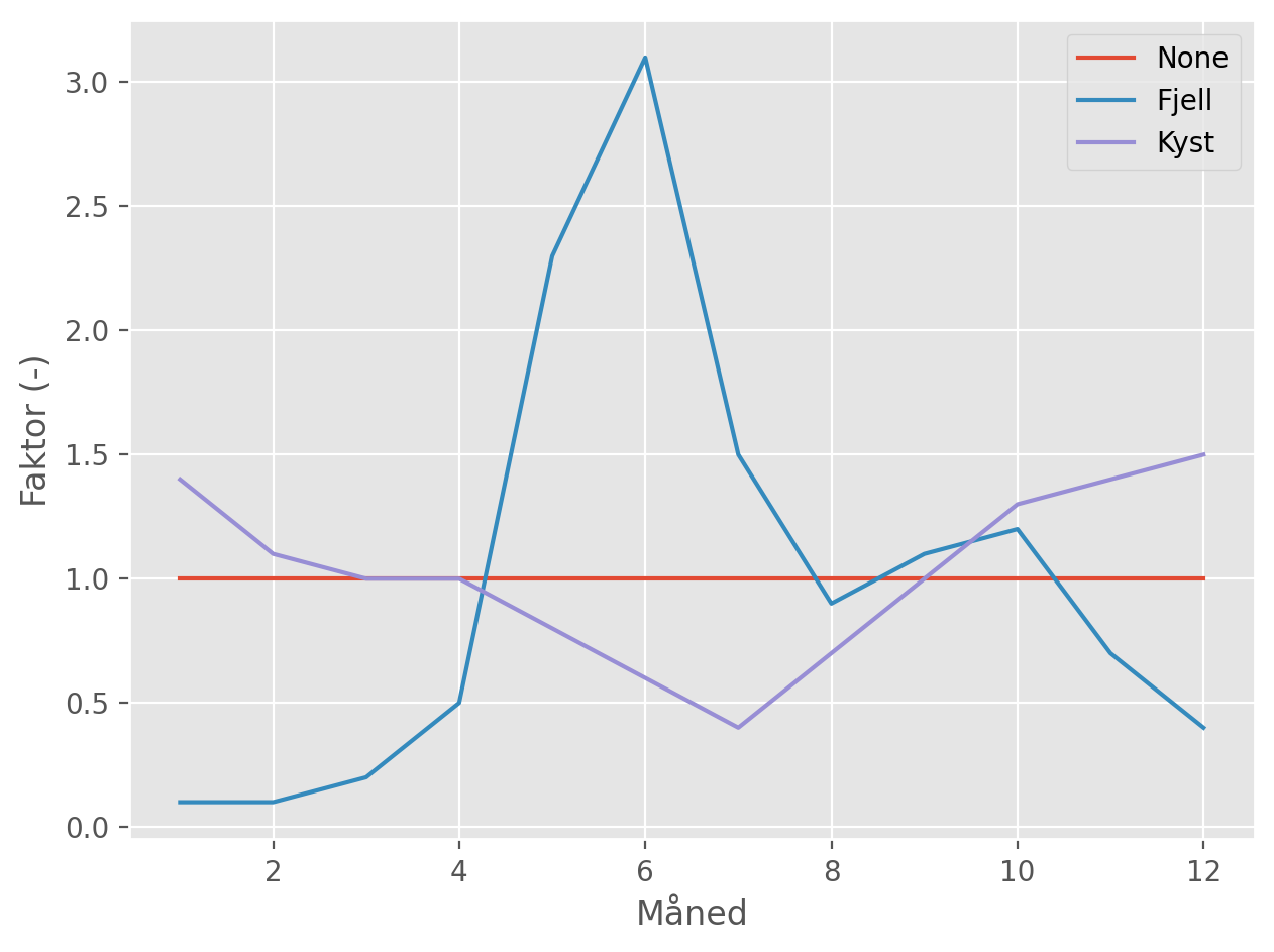
To avoid having to specify all these parameters when comparing different lime products, it is common to consider a standard lake with an area of 20 ha, mean depth of 5 m and mean residence time of 0.7 years. These parameters, in turn, define the mean annual discharge. If desired, this can be modified by selecting a monthly flow profile (fjell or kyst; see Figure 4), which adjusts the flows up or down in each month, but in such a way that the overall annual average maintains a residence time of 0.7 years.