Column tests
When lime is added to a lake, some of it dissolves quickly while the rest sinks to the bottom where it may dissolve more slowly. How much of the lime dissolves immediately depends on the lake chemistry, application method, and the properties of the lime product being used (see Lake modelling for details).
The proportion of a lime product that will dissolve “immediately” can be estimated using column tests (in this case, the term “immediately” means “within days”, rather than weeks, months or years). Each experiment involves 5 columns, labelled A to E. The columns are 19 cm in diameter and at least 205 cm high, and they are initially filled with 57.9 litres of deionised water containing 0.01% KCl, adjusted to the desired pH using sulphuric acid.
For each lime tested, the supplier must specify the typical proportions of Ca and Mg (by mass) in their product, \(F_{Ca}\) and \(F_{Mg}\). These fractions are used in the calculations below.
1 Instantaneous dissolution
For each type of lime, we would like to know the proportion that will dissolve “immediately” for a range of initial pH values and dose concentrations. The dose is usually expressed as a concentration in mg/l of lime i.e. the total mass of lime added, divided by the total volume of water in the column (or waterbody). If the dose concentration is \(D \ mg/l\) of lime and the proportion of calcium in the lime product by mass is \(F_{Ca}\), then if all the lime dissolves completely the concetration of Ca in the column will be \(F_{Ca} D \ mg/l\). The aim of the tests is to see how much of the lime actually dissolves under different conditions.
1.1 Varying pH
For the first set of tests, columns A to E are adjusted to have pH values of 4, 4.5, 5, 5.5 and 6, respectively. 0.579 g of dried lime are added to the top of each column, corresponding to a uniform dose of 10 mg/l of lime. If all of this dissolves and mixes evenly, the total mass of Ca or Mg dissolved in the column between any two depths \(x_1\) and \(x_2\) (where \(x_2 > x_1\)) is given by
\[ M_{par} = 10 F_{par} A (x_2 - x_1) \tag{1}\]
where \(A\) is the cross-sectional area of the column and \(par\) is either Ca or Mg.
In practice, not all the lime dissolves and the columns do not achieve uniform concentrations. After 16 hours, the concentration of Ca (and Mg, if relevant) in each column is determined at different depths using ICP-OES (Inductively Coupled Plasma - Optical Emission Spectrometry). Five measurements are taken from each column: every 40 cm from the surface down to 1.6 m. A typical dataset for a single column for a non-dolomitic lime (i.e. Ca only) is shown in Table 1.
| Column | pH | Depth (m) | Ca (mg/l) |
|---|---|---|---|
| A | 4.0 | 0.0 | 2.82 |
| A | 4.0 | 0.4 | 2.62 |
| A | 4.0 | 0.8 | 2.64 |
| A | 4.0 | 1.2 | 2.76 |
| A | 4.0 | 1.6 | 2.81 |
Table 1 is used to estimate the total amount of Ca that has actually dissolved in each column after 16 hours. It is assumed that each column is horizontally well-mixed and that concentrations only vary with depth, \(x\). The total amount of Ca between depths \(x_1\) and \(x_2\) is given by the integral
\[ M_{Ca} = A \int_{x_1}^{x_2} C(x) \ dx \tag{2}\]
The overall proportion of the available Ca that has dissolved, called the instantaneous dissolution, can then be obtained by dividing Equation 2 by Equation 1, both evaluated between 0 and 1.6 m depth (and the same calculation performed for magnesium, if relevant).
\[ D_{inst} = \frac{\int_{0}^{1.6} C(x) \ dx}{10 F_{Ca} (1.6 - 0)} \tag{3}\]
The integral in Equation 3 is approximated from the measured data (Table 1) using the trapezoidal rule.
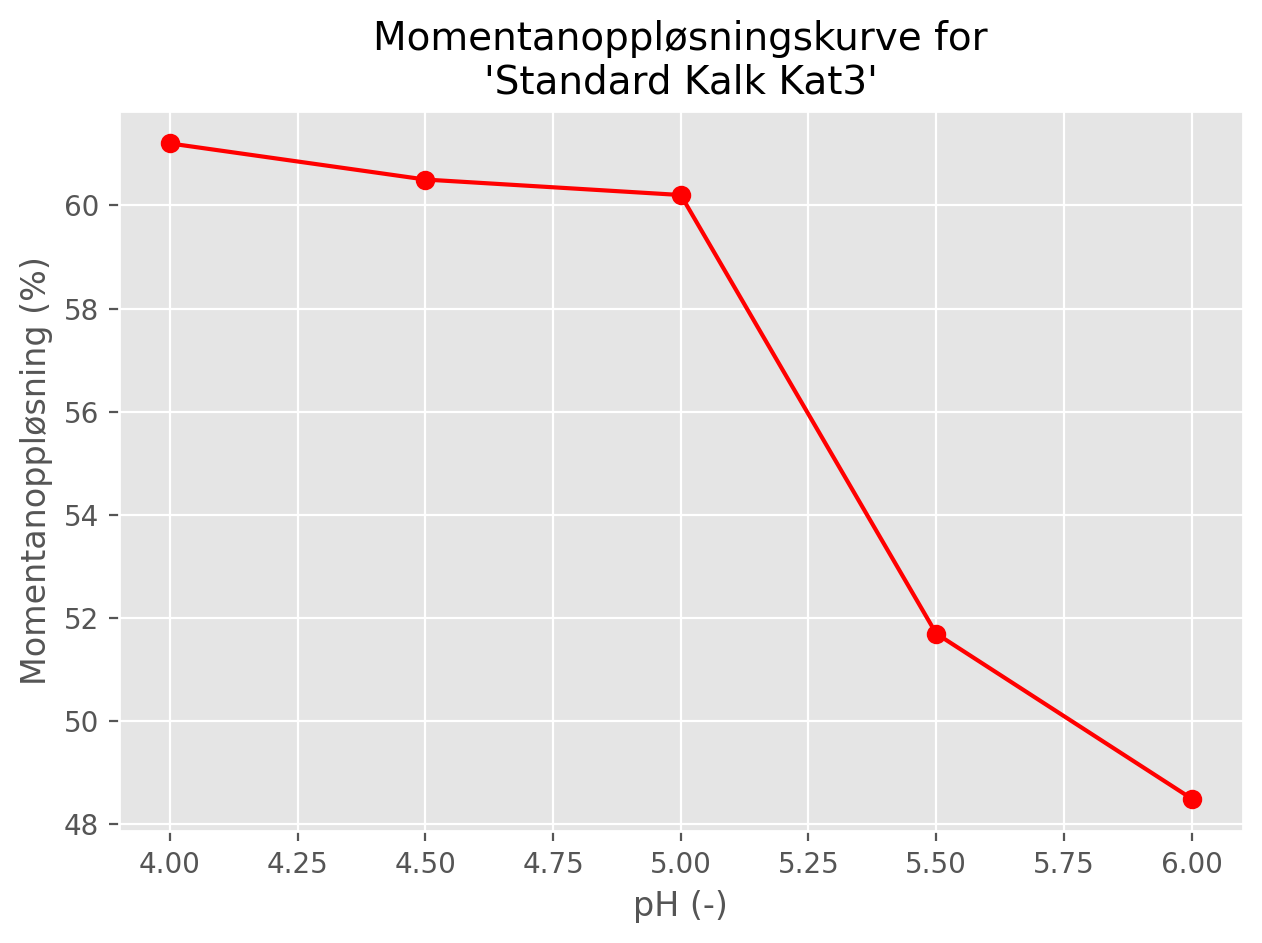
The main output from this experiment is a set instantaneous dissolution values (usually expressed in percent) showing how the dissolution changes with initial pH at a fixed lime dose (Figure 1).
1.2 Varying dose
In the second experiment, columns A to E are fixed at pH 4.5 and different doses are added to each column, corresponding to lime concentrations of 10, 20, 35, 50 and 85 mg/l (assuming complete dissolution). The columns are again left for 16 hours and the instantaneous dissolution for each column is determined using the procedure described in Section 1.1.
At high doses, the proportion of lime that dissolves immediately is typically lower than in the first experiment, because high doses lead to high calcium concentrations in the immediate vicinity of the lime particles, which inhibits dissolution. This effect is called overdosing.
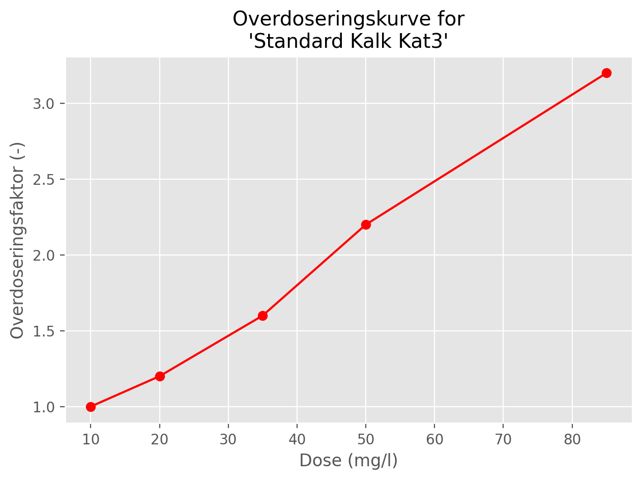
The main output from the second experiment is a set of overdosing factors, calculated as the ratio \(D_{10} / D_{x}\), where \(D_{10}\) is the instantaneous dissolution for the column where 10 mg/l of lime was initially added, and \(D_{x}\) is the instantaneous dissolution for the column where \(x\) mg/l of lime was added.
A typical curve for overdosing factors is shown in Figure 2.
1.3 Combining datasets
The two experiments described in Section 1.1 and Section 1.2 yield data in the format shown in Table 2.
x corresponds to a single column for which instantaneous dissolution is determined.
| pH Dose |
4 | 4.5 | 5 | 5.5 | 6 |
|---|---|---|---|---|---|
| 10 | x | x | x | x | x |
| 20 | x | ||||
| 35 | x | ||||
| 50 | x | ||||
| 85 | x |
Using these data, the expected instantaneous dissolution for any pH and lime dose can be estimated by interpolation.