The Mobius2 standard library
This is auto-generated documentation based on the Mobius2 standard library in Mobius2/stdlib .
The standard library provides common functions and constants for many models.
See the note on notation.
The file was generated at 2025-11-14 14:18:15.
Meteorology
File: stdlib/atmospheric.txt
Description
These are functions to derive various meteorological variables from more commonly measured variables. For use in e.g. estimation of potential evapotranspiration and air-sea heat fluxes.
They are mostly based on
Ventura, F., Spano, D., Duce, P. et al. An evaluation of common evapotranspiration equations. Irrig Sci 18, 163–170 (1999). https://doi.org/10.1007/s002710050058
See also
P. R. Lowe, 1977, An approximating polynomial for the computation of saturation vapor pressure, J. Appl. Meteor., 16, 100-103 https://doi.org/10.1175/1520-0450(1977)016<0100:AAPFTC>2.0.CO;2
Constants
| Name | Symbol | Unit | Value |
|---|---|---|---|
| Specific heat capacity of air | C_air | J kg⁻¹ K⁻¹ | 1008 |
| Specific heat capacity of moist air | C_moist_air | kJ kg⁻¹ K⁻¹ | 1.013 |
| Molar ratio to mass ratio of vapor in air | vapor_mol_to_mass | 0.62198 | |
| Specific gas constant of dry air | Rdry_air | J kg⁻¹ K⁻¹ | 287.058 |
| Specific gas constant of vapor | Rvap_air | J kg⁻¹ K⁻¹ | 461.495 |
Library functions
latent_heat_of_vaporization(T : °C) =
\[2.501 \mathrm{MJ}\,\mathrm{kg}^{-1}\,-0.002361 \mathrm{MJ}\,\mathrm{kg}^{-1}\,\mathrm{°C}^{-1}\,\cdot \mathrm{T}\]mean_barometric_pressure(elevation : m) =
\[\mathrm{elev} = \left(\mathrm{elevation}\Rightarrow 1\right) \\ \left(101.3-\left(0.01152-5.44\cdot 10^{7}\cdot \mathrm{elev}\right)\cdot \mathrm{elev}\Rightarrow \mathrm{kPa}\,\right)\]air_density(temp : °C, pressure : hPa, a_vap : hPa) =
\[\mathrm{tk} = \left(\mathrm{temp}\rightarrow \mathrm{K}\,\right) \\ \left(\frac{\mathrm{pressure}-\mathrm{a\_vap}}{\mathrm{tk}\cdot \mathrm{Rdry\_air}}+\frac{\mathrm{a\_vap}}{\mathrm{tk}\cdot \mathrm{Rvap\_air}}\rightarrow \mathrm{kg}\,\mathrm{m}^{-3}\,\right)\]psychrometric_constant(pressure : kPa, lvap : MJ kg⁻¹) =
\[\left(\mathrm{C\_moist\_air}\rightarrow \mathrm{MJ}\,\mathrm{kg}^{-1}\,\mathrm{K}^{-1}\,\right)\cdot \frac{\mathrm{pressure}}{\mathrm{vapor\_mol\_to\_mass}\cdot \mathrm{lvap}}\]saturation_vapor_pressure(T : °C) =
\[\mathrm{t} = \left(\mathrm{T}\Rightarrow 1\right) \\ \left(6.1078+\mathrm{t}\cdot \left(0.443652+\mathrm{t}\cdot \left(0.0142895+\mathrm{t}\cdot \left(0.000265065+\mathrm{t}\cdot \left(3.03124\cdot 10^{6}+\mathrm{t}\cdot \left(2.03408\cdot 10^{8}+\mathrm{t}\cdot 6.13682\cdot 10^{11}\right)\right)\right)\right)\right)\Rightarrow \mathrm{hPa}\,\right)\]slope_of_saturation_pressure_curve(T : °C, svap : kPa) =
\[\mathrm{tk} = \left(\mathrm{T}\rightarrow \mathrm{K}\,\right) \\ \frac{\mathrm{svap}}{\mathrm{tk}}\cdot \left(\frac{6790.5 \mathrm{K}\,}{\mathrm{tk}}-5.028\right)\]dew_point_temperature(vapor_pressure : hPa) =
\[34.07 \mathrm{K}\,+\frac{4157 \mathrm{K}\,}{\mathrm{ln}\left(\frac{2.1718\cdot 10^{8} \mathrm{hPa}\,}{\mathrm{vapor\_pressure}}\right)}\]specific_humidity_from_pressure(total_air_pressure : hPa, vapor_pressure : hPa) =
\[\mathrm{mixing\_ratio} = \mathrm{vapor\_mol\_to\_mass}\cdot \frac{\mathrm{vapor\_pressure}}{\mathrm{total\_air\_pressure}-\mathrm{vapor\_pressure}} \\ \frac{\mathrm{mixing\_ratio}}{1+\mathrm{mixing\_ratio}}\]Radiation
File: stdlib/atmospheric.txt
Description
This library provides functions for estimating solar radiation and downwelling longwave radiation.
The formulas are based on FAO paper 56
Constants
| Name | Symbol | Unit | Value |
|---|---|---|---|
| Solar constant | solar_constant | W m⁻² | 1361 |
Library functions
solar_declination(day_of_year : day) =
\[\mathrm{orbit\_rad} = \frac{2\cdot \pi\cdot \mathrm{day\_of\_year}}{365 \mathrm{day}\,} \\ 0.409\cdot \mathrm{sin}\left(\mathrm{orbit\_rad}-1.39\right)\]hour_angle(day_of_year : day, time_zone : hr, hour_of_day : hr, longitude : °) =
\[\mathrm{b} = 2\cdot \pi\cdot \frac{\mathrm{day\_of\_year}-81 \mathrm{day}\,}{365 \mathrm{day}\,} \\ \mathrm{eot} = \left(9.87\cdot \mathrm{sin}\left(2\cdot \mathrm{b}\right)-7.53\cdot \mathrm{cos}\left(\mathrm{b}\right)-1.5\cdot \mathrm{sin}\left(\mathrm{b}\right)\Rightarrow \mathrm{hr}\,\right) \\ \mathrm{lsmt} = 15 \mathrm{°}\,\mathrm{hr}^{-1}\,\cdot \mathrm{time\_zone} \\ \mathrm{ast} = \mathrm{hour\_of\_day}+\mathrm{eot}+\left(4 \mathrm{min}\,\mathrm{°}^{-1}\,\cdot \left(\mathrm{lsmt}-\mathrm{longitude}\right)\Rightarrow \mathrm{hr}\,\right) \\ \href{stdlib.html#basic}{\mathrm{radians}}\left(15 \mathrm{°}\,\mathrm{hr}^{-1}\,\cdot \left(\mathrm{ast}-12 \mathrm{hr}\,\right)\right)\]cos_zenith_angle(hour_a, day_of_year : day, latitude : °) =
\[\mathrm{lat\_rad} = \href{stdlib.html#basic}{\mathrm{radians}}\left(\mathrm{latitude}\right) \\ \mathrm{solar\_decl} = \href{stdlib.html#radiation}{\mathrm{solar\_declination}}\left(\mathrm{day\_of\_year}\right) \\ \mathrm{cz} = \mathrm{sin}\left(\mathrm{lat\_rad}\right)\cdot \mathrm{sin}\left(\mathrm{solar\_decl}\right)+\mathrm{cos}\left(\mathrm{lat\_rad}\right)\cdot \mathrm{cos}\left(\mathrm{solar\_decl}\right)\cdot \mathrm{cos}\left(\mathrm{hour\_a}\right) \\ \mathrm{max}\left(0,\, \mathrm{cz}\right)\]refract(cos_z, index) =
\[\sqrt{1-\frac{1-\mathrm{cos\_z}^{2}}{\mathrm{index}^{2}}}\]daily_average_extraterrestrial_radiation(latitude : °, day_of_year : day) =
\[\mathrm{orbit\_rad} = \frac{2\cdot \pi\cdot \mathrm{day\_of\_year}}{365 \mathrm{day}\,} \\ \mathrm{lat\_rad} = \href{stdlib.html#basic}{\mathrm{radians}}\left(\mathrm{latitude}\right) \\ \mathrm{solar\_decl} = \href{stdlib.html#radiation}{\mathrm{solar\_declination}}\left(\mathrm{day\_of\_year}\right) \\ \mathrm{sunset\_hour\_angle} = \mathrm{acos}\left(-\mathrm{tan}\left(\mathrm{lat\_rad}\right)\cdot \mathrm{tan}\left(\mathrm{solar\_decl}\right)\right) \\ \mathrm{inv\_rel\_dist\_earth\_sun} = 1+0.033\cdot \mathrm{cos}\left(\mathrm{orbit\_rad}\right) \\ \frac{\mathrm{solar\_constant}}{\pi}\cdot \mathrm{inv\_rel\_dist\_earth\_sun}\cdot \left(\mathrm{sunset\_hour\_angle}\cdot \mathrm{sin}\left(\mathrm{lat\_rad}\right)\cdot \mathrm{sin}\left(\mathrm{solar\_decl}\right)+\mathrm{cos}\left(\mathrm{lat\_rad}\right)\cdot \mathrm{cos}\left(\mathrm{solar\_decl}\right)\cdot \mathrm{sin}\left(\mathrm{sunset\_hour\_angle}\right)\right)\]hourly_average_radiation(daily_avg_rad : W m⁻², day_of_year : day, latitude : °, hour_angle) =
\[\mathrm{lat\_rad} = \href{stdlib.html#basic}{\mathrm{radians}}\left(\mathrm{latitude}\right) \\ \mathrm{solar\_decl} = \href{stdlib.html#radiation}{\mathrm{solar\_declination}}\left(\mathrm{day\_of\_year}\right) \\ \mathrm{sunset\_hour\_angle} = \mathrm{acos}\left(-\mathrm{tan}\left(\mathrm{lat\_rad}\right)\cdot \mathrm{tan}\left(\mathrm{solar\_decl}\right)\right) \\ \mathrm{cosshr} = \mathrm{cos}\left(\mathrm{sunset\_hour\_angle}\right) \\ \mathrm{factor} = \pi\cdot \frac{\mathrm{cos}\left(\mathrm{hour\_angle}\right)-\mathrm{cosshr}}{\mathrm{sin}\left(\mathrm{sunset\_hour\_angle}\right)-\mathrm{sunset\_hour\_angle}\cdot \mathrm{cosshr}} \\ \mathrm{daily\_avg\_rad}\cdot \mathrm{max}\left(0,\, \mathrm{factor}\right)\]clear_sky_shortwave(extrad : W m⁻², elev : m) =
\[\mathrm{extrad}\cdot \left(0.75+2\cdot 10^{5} \mathrm{m}^{-1}\,\cdot \mathrm{elev}\right)\]downwelling_longwave(air_temp : °C, a_vap : hPa, cloud) =
\[\mathrm{air\_t} = \left(\mathrm{air\_temp}\rightarrow \mathrm{K}\,\right) \\ \mathrm{dpt} = \href{stdlib.html#meteorology}{\mathrm{dew\_point\_temperature}}\left(\mathrm{a\_vap}\right) \\ \mathrm{dew\_point\_depression} = \mathrm{dpt}-\mathrm{air\_t} \\ \mathrm{cloud\_effect} = \left(10.77\cdot \mathrm{cloud}^{2}+2.34\cdot \mathrm{cloud}-18.44\Rightarrow \mathrm{K}\,\right) \\ \mathrm{vapor\_effect} = 0.84\cdot \left(\mathrm{dew\_point\_depression}+4.01 \mathrm{K}\,\right) \\ \mathrm{eff\_t} = \mathrm{air\_t}+\mathrm{cloud\_effect}+\mathrm{vapor\_effect} \\ \href{stdlib.html#thermodynamics}{\mathrm{black\_body\_radiation}}\left(\mathrm{eff\_t}\right)\]Basic constants
File: stdlib/physiochemistry.txt
Description
Some common physical constants.
Constants
| Name | Symbol | Unit | Value |
|---|---|---|---|
| Earth surface gravity | grav | m s⁻² | 9.81 |
Thermodynamics
File: stdlib/physiochemistry.txt
Description
Some common thermodynamic constants and functions.
Constants
| Name | Symbol | Unit | Value |
|---|---|---|---|
| Ideal gas constant | ideal_gas | J K⁻¹ mol⁻¹ | 8.31446 |
| Boltzmann constant | boltzmann | J K⁻¹ | 1.38065e-23 |
| Stefan-Boltzmann constant | stefan_boltzmann | W m⁻² K⁻⁴ | 5.67037e-08 |
Library functions
black_body_radiation(T : K) =
\[\mathrm{stefan\_boltzmann}\cdot \mathrm{T}^{4}\]enthalpy_adjust_log10(log10ref, ref_T : K, T : K, dU : kJ mol⁻¹) =
\[\mathrm{du} = \left(\mathrm{dU}\rightarrow \mathrm{J}\,\mathrm{mol}^{-1}\,\right) \\ \mathrm{log10ref}-\frac{\mathrm{du}}{\mathrm{ideal\_gas}\cdot \mathrm{ln}\left(10\right)}\cdot \left(\frac{1}{\mathrm{T}}-\frac{1}{\mathrm{ref\_T}}\right)\]Water utils
File: stdlib/physiochemistry.txt
Description
These are simplified functions for computing properties of freshwater at surface pressure. See the Seawater library for functions that take into account salinity and other factors.
References to be inserted.
Constants
| Name | Symbol | Unit | Value |
|---|---|---|---|
| Water density | rho_water | kg m⁻³ | 999.98 |
| Specific heat capacity of water | C_water | J kg⁻¹ K⁻¹ | 4186 |
| Thermal conductivity of water | k_water | W m⁻¹ K⁻¹ | 0.6 |
| Refraction index of water | refraction_index_water | 1.33 | |
| Refraction index of ice | refraction_index_ice | 1.31 |
Library functions
water_temp_to_heat(V : m³, T : °C) =
\[\mathrm{V}\cdot \left(\mathrm{T}\rightarrow \mathrm{K}\,\right)\cdot \mathrm{rho\_water}\cdot \mathrm{C\_water}\]water_heat_to_temp(V : m³, heat : J) =
\[\left(\frac{\mathrm{heat}}{\mathrm{V}\cdot \mathrm{rho\_water}\cdot \mathrm{C\_water}}\rightarrow \mathrm{°C}\,\right)\]water_density(T : °C) =
\[\mathrm{dtemp} = \left(\mathrm{T}\rightarrow \mathrm{K}\,\right)-277.13 \mathrm{K}\, \\ \mathrm{rho\_water}\cdot \left(1-0.5\cdot 1.6509\cdot 10^{5} \mathrm{K}^{-2}\,\cdot \mathrm{dtemp}^{2}\right)\]dynamic_viscosity_water(T : K) =
\[2646.8 \mathrm{g}\,\mathrm{m}^{-1}\,\mathrm{s}^{-1}\,\cdot e^{\left(-0.0268\cdot \mathrm{T}\Rightarrow 1\right)}\]kinematic_viscosity_water(T : K) =
\[0.00285 \mathrm{m}^{2}\,\mathrm{s}^{-1}\,\cdot e^{\left(-0.027\cdot \mathrm{T}\Rightarrow 1\right)}\]Diffusivity
File: stdlib/physiochemistry.txt
Description
This library contains functions for computing diffusivities of compounds in water and air.
Reference: Schwarzengack, Gschwend, Imboden, “Environmental organic chemistry” 2nd ed https://doi.org/10.1002/0471649643.
Constants
| Name | Symbol | Unit | Value |
|---|---|---|---|
| Molecular volume of air at surface pressure | molvol_air | cm³ mol⁻¹ | 20.1 |
| Molecular mass of air | molmass_air | g mol⁻¹ | 28.97 |
| Molecular volume of H2O vapour at surface pressure | molvol_h2o | cm³ mol⁻¹ | 22.41 |
| Molecular mass of H2O | molmass_h2o | g mol⁻¹ | 18 |
Library functions
molecular_diffusivity_of_compound_in_air(mol_vol : cm³ mol⁻¹, mol_mass : g mol⁻¹, T : K) =
\[\mathrm{TT} = \left(\mathrm{T}\Rightarrow 1\right) \\ \mathrm{c0} = \sqrt[3]{\left(\mathrm{molvol\_air}\Rightarrow 1\right)}+\sqrt[3]{\left(\mathrm{mol\_vol}\Rightarrow 1\right)} \\ \mathrm{c} = \frac{\sqrt{\frac{1}{\left(\mathrm{molmass\_air}\Rightarrow 1\right)}+\frac{1}{\left(\mathrm{mol\_mass}\Rightarrow 1\right)}}}{\mathrm{c0}^{2}} \\ \left(10^{-7}\cdot \mathrm{c}\cdot \mathrm{TT}^{1.75}\Rightarrow \mathrm{m}^{2}\,\mathrm{s}^{-1}\,\right)\]molecular_diffusivity_of_compound_in_water(mol_vol : cm³ mol⁻¹, dynamic_viscosity : g m⁻¹ s⁻¹) =
\[\mathrm{dynv} = \left(\mathrm{dynamic\_viscosity}\Rightarrow 1\right) \\ \frac{1.326\cdot 10^{8} \mathrm{m}^{2}\,\mathrm{s}^{-1}\,}{\mathrm{dynv}^{1.14}\cdot \left(\mathrm{mol\_vol}\Rightarrow 1\right)^{0.589}}\]diffusion_velocity_of_vapour_in_air(wind : m s⁻¹) =
\[0.002\cdot \mathrm{wind}+0.003 \mathrm{m}\,\mathrm{s}^{-1}\,\]transfer_velocity_of_CO2_in_water_20C(wind : m s⁻¹) =
\[\mathrm{w} = \left(\mathrm{wind}\Rightarrow 1\right) \\ \left(\begin{cases}0.00065 & \text{if}\;\mathrm{w}\leq 4.2 \\ \left(0.79\cdot \mathrm{w}-2.68\right)\cdot 0.001 & \text{if}\;\mathrm{w}\leq 13 \\ \left(1.64\cdot \mathrm{w}-13.69\right)\cdot 0.001 & \text{otherwise}\end{cases}\Rightarrow \mathrm{cm}\,\mathrm{s}^{-1}\,\right)\]waterside_vel_low_turbulence(T : K, moldiff : m² s⁻¹, wind : m s⁻¹) =
\[\mathrm{kinvis} = \href{stdlib.html#water-utils}{\mathrm{kinematic\_viscosity\_water}}\left(\mathrm{T}\right) \\ \mathrm{schmidt} = \frac{\mathrm{kinvis}}{\mathrm{moldiff}} \\ \mathrm{asc} = \begin{cases}0.67 & \text{if}\;\mathrm{wind}<4.2 \mathrm{m}\,\mathrm{s}^{-1}\, \\ 0.5 & \text{otherwise}\end{cases} \\ \mathrm{vCO2} = \href{stdlib.html#diffusivity}{\mathrm{transfer\_velocity\_of\_CO2\_in\_water\_20C}}\left(\mathrm{wind}\right) \\ \left(\left(\frac{\mathrm{schmidt}}{600}\right)^{-\mathrm{asc}}\cdot \mathrm{vCO2}\rightarrow \mathrm{m}\,\mathrm{s}^{-1}\,\right)\]Chemistry
File: stdlib/physiochemistry.txt
Description
This library contains some commonly used molar masses and functions to convert molar ratios to mass ratios.
Constants
| Name | Symbol | Unit | Value |
|---|---|---|---|
| O₂ molar mass | o2_mol_mass | g mol⁻¹ | 31.998 |
| C molar mass | c_mol_mass | g mol⁻¹ | 12 |
| N molar mass | n_mol_mass | g mol⁻¹ | 14.01 |
| P molar mass | p_mol_mass | g mol⁻¹ | 30.97 |
| NO₃ molar mass | no3_mol_mass | g mol⁻¹ | 62 |
| PO₄ molar mass | po4_mol_mass | g mol⁻¹ | 94.9714 |
| Ca molar mass | ca_mol_mass | g mol⁻¹ | 40.078 |
| CH₄ molar mass | ch4_mol_mass | g mol⁻¹ | 16.04 |
Library functions
nc_molar_to_mass_ratio(nc_molar) =
\[\mathrm{nc\_molar}\cdot \frac{\mathrm{n\_mol\_mass}}{\mathrm{c\_mol\_mass}}\]pc_molar_to_mass_ratio(pc_molar) =
\[\mathrm{pc\_molar}\cdot \frac{\mathrm{p\_mol\_mass}}{\mathrm{c\_mol\_mass}}\]cn_molar_to_mass_ratio(cn_molar) =
\[\mathrm{cn\_molar}\cdot \frac{\mathrm{c\_mol\_mass}}{\mathrm{n\_mol\_mass}}\]cp_molar_to_mass_ratio(cp_molar) =
\[\mathrm{cp\_molar}\cdot \frac{\mathrm{c\_mol\_mass}}{\mathrm{p\_mol\_mass}}\]Basic
File: stdlib/basic_math.txt
Description
This library provides some very common math functions.
Library functions
safe_divide(a, b) =
\[\mathrm{r} = \frac{\mathrm{a}}{\mathrm{b}} \\ \begin{cases}\mathrm{r} & \text{if}\;\mathrm{is\_finite}\left(\mathrm{r}\right) \\ 0 & \text{otherwise}\end{cases}\]close(a, b, tol) =
\[\left|\mathrm{a}-\mathrm{b}\right|<\mathrm{tol}\]clamp(a, mn, mx) =
\[\mathrm{min}\left(\mathrm{max}\left(\mathrm{a},\, \mathrm{mn}\right),\, \mathrm{mx}\right)\]radians(a : °) =
\[\mathrm{a}\cdot \frac{\pi}{180 \mathrm{°}\,}\]Response
File: stdlib/basic_math.txt
Description
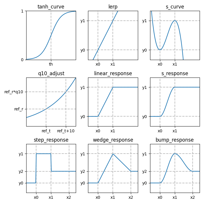
This library provides functions that let some state respond to another state. For instance,
q10_adjust creates a Q10 response of a reference rate to a temperature.
The various response functions allow you to interpolate a value \(y\) between different levels \(y_0\), \(y_1\), …, depending on an input variable \(x\) and thresholds \(x_0\), \(x_1\), etc.
Library functions
hl_to_rate(hl) =
\[\frac{\mathrm{ln}\left(2\right)}{\mathrm{hl}}\]rate_to_hl(rate) =
\[\frac{\mathrm{ln}\left(2\right)}{\mathrm{rate}}\]q10_adjust(ref_rate, ref_temp : °C, temp : °C, q10) =
\[\mathrm{ref\_rate}\cdot \mathrm{q10}^{\frac{\mathrm{temp}-\mathrm{ref\_temp}}{10 \mathrm{°C}\,}}\]lerp(x, x0, x1, y0, y1) =
\[\mathrm{t} = \frac{\mathrm{x}-\mathrm{x0}}{\mathrm{x1}-\mathrm{x0}} \\ \left(1-\mathrm{t}\right)\cdot \mathrm{y0}+\mathrm{t}\cdot \mathrm{y1}\]s_curve(x, x0, x1, y0, y1) =
\[\mathrm{t} = \frac{\mathrm{x}-\mathrm{x0}}{\mathrm{x1}-\mathrm{x0}} \\ \mathrm{tt} = \left(3-2\cdot \mathrm{t}\right)\cdot \mathrm{t}^{2} \\ \left(1-\mathrm{tt}\right)\cdot \mathrm{y0}+\mathrm{tt}\cdot \mathrm{y1}\]tanh_curve(x, th) =
\[0.5\cdot \left(1+\mathrm{tanh}\left(\mathrm{x}-\mathrm{th}\right)\right)\]linear_response(x, x0, x1, y0, y1) =
\[\begin{cases}\mathrm{y0} & \text{if}\;\mathrm{x}\leq \mathrm{x0} \\ \mathrm{y1} & \text{if}\;\mathrm{x}\geq \mathrm{x1} \\ \href{stdlib.html#response}{\mathrm{lerp}}\left(\mathrm{x},\, \mathrm{x0},\, \mathrm{x1},\, \mathrm{y0},\, \mathrm{y1}\right) & \text{otherwise}\end{cases}\]s_response(x, x0, x1, y0, y1) =
\[\begin{cases}\mathrm{y0} & \text{if}\;\mathrm{x}\leq \mathrm{x0} \\ \mathrm{y1} & \text{if}\;\mathrm{x}\geq \mathrm{x1} \\ \href{stdlib.html#response}{\mathrm{s\_curve}}\left(\mathrm{x},\, \mathrm{x0},\, \mathrm{x1},\, \mathrm{y0},\, \mathrm{y1}\right) & \text{otherwise}\end{cases}\]step_response(x, x0, x1, y0, y1, y2) =
\[\begin{cases}\mathrm{y0} & \text{if}\;\mathrm{x}\leq \mathrm{x0} \\ \mathrm{y1} & \text{if}\;\mathrm{x}\leq \mathrm{x1} \\ \mathrm{y2} & \text{otherwise}\end{cases}\]wedge_response(x, x0, x1, x2, y0, y1, y2) =
\[\begin{cases}\mathrm{y0} & \text{if}\;\mathrm{x}\leq \mathrm{x0} \\ \mathrm{y2} & \text{if}\;\mathrm{x}\geq \mathrm{x2} \\ \href{stdlib.html#response}{\mathrm{lerp}}\left(\mathrm{x},\, \mathrm{x0},\, \mathrm{x1},\, \mathrm{y0},\, \mathrm{y1}\right) & \text{if}\;\mathrm{x}\leq \mathrm{x1} \\ \href{stdlib.html#response}{\mathrm{lerp}}\left(\mathrm{x},\, \mathrm{x1},\, \mathrm{x2},\, \mathrm{y1},\, \mathrm{y2}\right) & \text{otherwise}\end{cases}\]bump_response(x, x0, x1, x2, y0, y1, y2) =
\[\begin{cases}\mathrm{y0} & \text{if}\;\mathrm{x}\leq \mathrm{x0} \\ \mathrm{y2} & \text{if}\;\mathrm{x}\geq \mathrm{x2} \\ \href{stdlib.html#response}{\mathrm{s\_curve}}\left(\mathrm{x},\, \mathrm{x0},\, \mathrm{x1},\, \mathrm{y0},\, \mathrm{y1}\right) & \text{if}\;\mathrm{x}\leq \mathrm{x1} \\ \href{stdlib.html#response}{\mathrm{s\_curve}}\left(\mathrm{x},\, \mathrm{x1},\, \mathrm{x2},\, \mathrm{y1},\, \mathrm{y2}\right) & \text{otherwise}\end{cases}\]Air-sea
File: stdlib/seawater.txt
Description
Air-sea/lake heat fluxes are based off of Air-Sea bulk transfer coefficients in diabatic conditions, Junsei Kondo, 1975, Boundary-Layer Meteorology 9(1), 91-112 https://doi.org/10.1007/BF00232256
The implementation used here is influenced by the implementation in GOTM.
Library functions
surface_stability(wind : m s⁻¹, water_temp : °C, air_temp : °C) =
\[\mathrm{ww} = \mathrm{wind}+10^{-10} \mathrm{m}\,\mathrm{s}^{-1}\, \\ \mathrm{s0} = \left(0.25\cdot \frac{\mathrm{water\_temp}-\mathrm{air\_temp}}{\mathrm{ww}\cdot \mathrm{ww}}\Rightarrow 1\right) \\ \mathrm{s0}\cdot \frac{\left|\mathrm{s0}\right|}{\left|\mathrm{s0}\right|+0.01}\]stab_modify(wind : m s⁻¹, stab) =
\[\begin{cases}0 & \text{if}\;\left|\mathrm{wind}\right|<0.001 \mathrm{m}\,\mathrm{s}^{-1}\, \\ 0.1+0.03\cdot \mathrm{stab}\cdot 0.9\cdot e^{4.8\cdot \mathrm{stab}} & \text{if}\;\mathrm{stab}<0\;\text{and}\;\mathrm{stab}>-3.3 \\ 0 & \text{if}\;\mathrm{stab}<0 \\ 1+0.63\cdot \sqrt{\mathrm{stab}} & \text{otherwise}\end{cases}\]tc_latent_heat(wind : m s⁻¹, stability) =
\[\mathrm{w} = \left(\mathrm{wind}\Rightarrow 1\right)+10^{-12} \\ \left(\begin{cases}0+1.23\cdot e^{-0.16\cdot \mathrm{ln}\left(\mathrm{w}\right)} & \text{if}\;\mathrm{w}<2.2 \\ 0.969+0.0521\cdot \mathrm{w} & \text{if}\;\mathrm{w}<5 \\ 1.18+0.01\cdot \mathrm{w} & \text{if}\;\mathrm{w}<8 \\ 1.196+0.008\cdot \mathrm{w}-0.0004\cdot \left(\mathrm{w}-8\right)^{2} & \text{if}\;\mathrm{w}<25 \\ 1.68-0.016\cdot \mathrm{w} & \text{otherwise}\end{cases}\right)\cdot 0.001\cdot \href{stdlib.html#air-sea}{\mathrm{stab\_modify}}\left(\mathrm{wind},\, \mathrm{stability}\right)\]tc_sensible_heat(wind : m s⁻¹, stability) =
\[\mathrm{w} = \left(\mathrm{wind}\Rightarrow 1\right)+10^{-12} \\ \left(\begin{cases}0+1.185\cdot e^{-0.157\cdot \mathrm{ln}\left(\mathrm{w}\right)} & \text{if}\;\mathrm{w}<2.2 \\ 0.927+0.0546\cdot \mathrm{w} & \text{if}\;\mathrm{w}<5 \\ 1.15+0.01\cdot \mathrm{w} & \text{if}\;\mathrm{w}<8 \\ 1.17+0.0075\cdot \mathrm{w}-0.00045\cdot \left(\mathrm{w}-8\right)^{2} & \text{if}\;\mathrm{w}<25 \\ 1.652-0.017\cdot \mathrm{w} & \text{otherwise}\end{cases}\right)\cdot 0.001\cdot \href{stdlib.html#air-sea}{\mathrm{stab\_modify}}\left(\mathrm{wind},\, \mathrm{stability}\right)\]Seawater
File: stdlib/seawater.txt
Description
This is a library for highly accurate, but more computationally expensive, properties of sea water (taking salinity into account). Se the library Water utils for simplified freshwater versions of these functions.
The formulas for density are taken from the Matlab seawater package.
The formulas for viscosity and diffusivity are taken from
Riley, J. P. & Skirrow, G. Chemical oceanography. 2 edn, Vol. 1 606 (Academic Press, 1975).
Constants
| Name | Symbol | Unit | Value |
|---|---|---|---|
| Ice formation temperature salinity dependence | fr_t_s | °C | 0.056 |
Library functions
ice_formation_temperature(S) =
\[-\mathrm{S}\cdot \mathrm{fr\_t\_s}\]seawater_dens_standard_mean(T : °C) =
\[\mathrm{a0} = 999.843 \\ \mathrm{a1} = 0.0679395 \\ \mathrm{a2} = -0.00909529 \\ \mathrm{a3} = 0.000100169 \\ \mathrm{a4} = -1.12008\cdot 10^{6} \\ \mathrm{a5} = 6.53633\cdot 10^{9} \\ \mathrm{T68} = \left(\mathrm{T}\cdot 1.00024\Rightarrow 1\right) \\ \left(\mathrm{a0}+\left(\mathrm{a1}+\left(\mathrm{a2}+\left(\mathrm{a3}+\left(\mathrm{a4}+\mathrm{a5}\cdot \mathrm{T68}\right)\cdot \mathrm{T68}\right)\cdot \mathrm{T68}\right)\cdot \mathrm{T68}\right)\cdot \mathrm{T68}\Rightarrow \mathrm{kg}\,\mathrm{m}^{-3}\,\right)\]seawater_pot_dens(T : °C, S) =
\[\mathrm{b0} = 0.824493 \\ \mathrm{b1} = -0.0040899 \\ \mathrm{b2} = 7.6438\cdot 10^{5} \\ \mathrm{b3} = -8.2467\cdot 10^{7} \\ \mathrm{b4} = 5.3875\cdot 10^{9} \\ \mathrm{c0} = -0.00572466 \\ \mathrm{c1} = 0.00010227 \\ \mathrm{c2} = -1.6546\cdot 10^{6} \\ \mathrm{d0} = 0.00048314 \\ \mathrm{T68} = \left(\mathrm{T}\cdot 1.00024\Rightarrow 1\right) \\ \href{stdlib.html#seawater}{\mathrm{seawater\_dens\_standard\_mean}}\left(\mathrm{T}\right)+\left(\left(\mathrm{b0}+\left(\mathrm{b1}+\left(\mathrm{b2}+\left(\mathrm{b3}+\mathrm{b4}\cdot \mathrm{T68}\right)\cdot \mathrm{T68}\right)\cdot \mathrm{T68}\right)\cdot \mathrm{T68}\right)\cdot \mathrm{S}+\left(\mathrm{c0}+\left(\mathrm{c1}+\mathrm{c2}\cdot \mathrm{T68}\right)\cdot \mathrm{T68}\right)\cdot \mathrm{S}\cdot \sqrt{\mathrm{S}}+\mathrm{d0}\cdot \mathrm{S}^{2}\Rightarrow \mathrm{kg}\,\mathrm{m}^{-3}\,\right)\]dynamic_viscosity_fresh_water(T : °C) =
\[\mathrm{eta20} = 0.001002 \mathrm{Pa}\,\mathrm{s}\, \\ \mathrm{tm20} = 20 \mathrm{°C}\,-\mathrm{T} \\ \mathrm{lograt} = \frac{1.1709\cdot \mathrm{tm20}-0.001827 \mathrm{°C}^{-1}\,\cdot \mathrm{tm20}^{2}}{\mathrm{T}+89.93 \mathrm{°C}\,} \\ \mathrm{eta20}\cdot 10^{\mathrm{lograt}}\]dynamic_viscosity_sea_water(T : °C, S) =
\[\mathrm{eta\_t} = \href{stdlib.html#seawater}{\mathrm{dynamic\_viscosity\_fresh\_water}}\left(\mathrm{T}\right) \\ \mathrm{a} = \href{stdlib.html#response}{\mathrm{lerp}}\left(\mathrm{T},\, 5 \mathrm{°C}\,,\, 25 \mathrm{°C}\,,\, 0.000366,\, 0.001403\right) \\ \mathrm{b} = \href{stdlib.html#response}{\mathrm{lerp}}\left(\mathrm{T},\, 5 \mathrm{°C}\,,\, 25 \mathrm{°C}\,,\, 0.002756,\, 0.003416\right) \\ \mathrm{cl} = \mathrm{max}\left(0,\, \frac{\mathrm{S}-0.03}{1.805}\right) \\ \mathrm{clv} = \left(\href{stdlib.html#seawater}{\mathrm{seawater\_pot\_dens}}\left(\mathrm{T},\, \mathrm{S}\right)\cdot \mathrm{cl}\Rightarrow 1\right) \\ \mathrm{eta\_t}\cdot \left(1+\mathrm{a}\cdot \sqrt{\mathrm{clv}}+\mathrm{b}\cdot \mathrm{clv}\right)\]diffusivity_in_water(ref_diff, ref_T : °C, ref_S, T : °C, S) =
\[\mathrm{ref\_diff}\cdot \frac{\href{stdlib.html#seawater}{\mathrm{dynamic\_viscosity\_sea\_water}}\left(\mathrm{ref\_T},\, \mathrm{ref\_S}\right)}{\href{stdlib.html#seawater}{\mathrm{dynamic\_viscosity\_sea\_water}}\left(\mathrm{T},\, \mathrm{S}\right)}\cdot \frac{\left(\mathrm{T}\rightarrow \mathrm{K}\,\right)}{\left(\mathrm{ref\_T}\rightarrow \mathrm{K}\,\right)}\]Sea oxygen
File: stdlib/seawater.txt
Description
This contains formulas for O₂, CO₂ and CH₄ saturation and surface exchange in sea water. Based on
R.F. Weiss, The solubility of nitrogen, oxygen and argon in water and seawater, Deep Sea Research and Oceanographic Abstracts, Volume 17, Issue 4, 1970, 721-735, https://doi.org/10.1016/0011-7471(70)90037-9.
The implementation is influenced by the one in SELMA.
There are other undocumented sources. This should be updated soon.
Library functions
o2_saturation_concentration(T : °C, S) =
\[\mathrm{Tk} = \left(\left(\mathrm{T}\rightarrow \mathrm{K}\,\right)\Rightarrow 1\right) \\ \mathrm{logsat} = -135.902+\frac{157570}{\mathrm{Tk}}-\frac{6.64231\cdot 10^{7}}{\mathrm{Tk}^{2}}+\frac{1.2438\cdot 10^{10}}{\mathrm{Tk}^{3}}-\frac{8.62195\cdot 10^{11}}{\mathrm{Tk}^{4}}-\mathrm{S}\cdot \left(0.017674-\frac{10.754}{\mathrm{Tk}}+\frac{2140.7}{\mathrm{Tk}^{2}}\right) \\ \left(e^{\mathrm{logsat}}\Rightarrow \mathrm{mmol}\,\mathrm{m}^{-3}\,\right)\]co2_saturation_concentration(T : °C, co2_atm_ppm, air_pressure) =
\[\mathrm{Tk} = \left(\left(\mathrm{T}\rightarrow \mathrm{K}\,\right)\Rightarrow 1\right) \\ \mathrm{log10Kh} = 108.386+0.0198508\cdot \mathrm{Tk}-\frac{6919.53}{\mathrm{Tk}}-40.4515\cdot \mathrm{log}_{10}\left(\mathrm{Tk}\right)+\frac{669365}{\mathrm{Tk}^{2}} \\ \mathrm{Kh} = \left(10^{\mathrm{log10Kh}}\Rightarrow \mathrm{mol}\,\mathrm{l}^{-1}\,\mathrm{bar}^{-1}\,\right) \\ \mathrm{pCO2} = \mathrm{co2\_atm\_ppm}\cdot 10^{-6}\cdot \mathrm{air\_pressure} \\ \left(\mathrm{pCO2}\cdot \mathrm{Kh}\cdot \mathrm{c\_mol\_mass}\rightarrow \mathrm{mg}\,\mathrm{l}^{-1}\,\right)\]ch4_saturation_concentration(T : °C, ch4_atm_ppm, air_pressure) =
\[\mathrm{Tk} = \left(\left(\mathrm{T}\rightarrow \mathrm{K}\,\right)\Rightarrow 1\right) \\ \mathrm{Kh} = \left(\frac{e^{\frac{-365.183+\frac{18103.7}{\mathrm{Tk}}+49.7554\cdot \mathrm{ln}\left(\mathrm{Tk}\right)-0.000285033\cdot \mathrm{Tk}}{1.9872}}}{55.556}\Rightarrow \mathrm{mol}\,\mathrm{l}^{-1}\,\mathrm{bar}^{-1}\,\right) \\ \mathrm{pCH4} = \mathrm{ch4\_atm\_ppm}\cdot 10^{-6}\cdot \mathrm{air\_pressure} \\ \left(\mathrm{pCH4}\cdot \mathrm{Kh}\cdot \mathrm{ch4\_mol\_mass}\rightarrow \mathrm{mg}\,\mathrm{l}^{-1}\,\right)\]schmidt_600(wind : m s⁻¹) =
\[\mathrm{wnd} = \left(\mathrm{wind}\Rightarrow 1\right) \\ 2.07+0.215\cdot \mathrm{wnd}^{1.7}\]o2_piston_velocity(wind : m s⁻¹, temp : °C) =
\[\mathrm{T} = \left(\mathrm{temp}\Rightarrow 1\right) \\ \mathrm{k\_600} = \href{stdlib.html#sea-oxygen}{\mathrm{schmidt\_600}}\left(\mathrm{wind}\right) \\ \mathrm{schmidt} = 1800.6-120.1\cdot \mathrm{T}+3.7818\cdot \mathrm{T}^{2}-0.047608\cdot \mathrm{T}^{3} \\ \left(\mathrm{k\_600}\cdot \left(\frac{\mathrm{schmidt}}{600}\right)^{-0.666}\Rightarrow \mathrm{cm}\,\mathrm{hr}^{-1}\,\right)\]co2_piston_velocity(wind : m s⁻¹, temp : °C) =
\[\mathrm{T} = \left(\mathrm{temp}\Rightarrow 1\right) \\ \mathrm{k\_600} = \href{stdlib.html#sea-oxygen}{\mathrm{schmidt\_600}}\left(\mathrm{wind}\right) \\ \mathrm{schmidt} = 1923.6-125.06\cdot \mathrm{T}+4.3773\cdot \mathrm{T}^{2}-0.085681\cdot \mathrm{T}^{3}+0.00070284\cdot \mathrm{T}^{4} \\ \left(\mathrm{k\_600}\cdot \mathrm{min}\left(2.5,\, \left(\frac{\mathrm{schmidt}}{600}\right)^{-0.666}\right)\Rightarrow \mathrm{cm}\,\mathrm{hr}^{-1}\,\right)\]ch4_piston_velocity(wind : m s⁻¹, temp : °C) =
\[\mathrm{T} = \left(\mathrm{temp}\Rightarrow 1\right) \\ \mathrm{k\_600} = \href{stdlib.html#sea-oxygen}{\mathrm{schmidt\_600}}\left(\mathrm{wind}\right) \\ \mathrm{schmidt} = 1909.4-120.78\cdot \mathrm{T}+4.1555\cdot \mathrm{T}^{2}-0.080578\cdot \mathrm{T}^{3}+0.00065777\cdot \mathrm{T}^{4} \\ \left(\mathrm{k\_600}\cdot \mathrm{min}\left(2.5,\, \left(\frac{\mathrm{schmidt}}{600}\right)^{-0.666}\right)\Rightarrow \mathrm{cm}\,\mathrm{hr}^{-1}\,\right)\]