2. The TEOTIL model
2.1. Development history
The original TEOTIL model was created in 1992 (Ibrekk and Tjomsland, 1992). In 2001, it was recoded into Visual Basic and, in 2017, the code was refactored again into Python — a language that is increasingly popular for scientific applications. The Python implementation of the model currently lacks a graphical user interface, but it is more flexible and efficient than the previous version, making it feasible to extend the model to other parameters while also reducing runtimes.
2.2. Nitrogen and phosphorus
The purpose of the existing TEOTIL model is to integrate nutrient inputs from a variety of sources and to accumulate them downstream. Key datasets for simulating nitrogen and phosphorus include: diffuse background inputs from forests & uplands; diffuse human inputs based on population density & agricultural activities; and point discharges from industry, sewage treatment & aquaculture. The model uses the “export coefficient” concept to estimate diffuse fluxes, and it also incorporates a simple representation of catchment-level nutrient cycling and retention. For national scale applications, the model typically uses the “regine” catchment network, which comprises roughly 20 000 sub-catchments across Norway, ranging in size between 0.01 and 10 000 km².
2.3. Model structure and constraints
Extending TEOTIL to incorporate additional parameters requires understanding the model’s structural framework, which places constraints upon further development. To simulate fluxes for any given parameter, \(X\), the model must perform the following calculations:
-
Sum “local” inputs of \(X\) for each sub-catchment. In the case of N and P, diffuse inputs are estimated by applying export coefficients to datasets of land use and agricultural activities in each catchment. These are then added to the sum of all point discharges located within the catchment boundary to give the total local input of \(X\) to catchment \(i\), denoted \(L_i^X\)
-
Accumulate loads downstream. Each sub-catchment, \(i\), is assigned a parameter-specific retention factor, \(\alpha_i^X\), between 0 and 1. This indicates the proportion of the load of \(X\) entering the catchment that is retained due to internal cycling.
The model begins by identifying the uppermost sub-catchment(s) in each river system. For these headwater catchments, the amount of \(X\) transmitted to the next catchment downstream is
\[T_i^X=(1 - \alpha_i^X ) L_i^X \quad \quad \quad (1)\]For the next catchment downstream, \(j\), the total input of \(X\) is equal to the sum of local sources, \(L_j^X\), plus any inputs from catchments upstream (numbered 1 to \(n\) in equation [2], below). The output from catchment \(j\) is therefore
\[T_j^X=(1 - \alpha_j^X )\left(L_j^X + \sum_{p=1}^nT_p^X\right) \quad \quad \quad (2)\]These calculations are illustrated schematically in Fig. 1. Adding additional chemical species to TEOTIL therefore requires estimating two parameters per species for each sub-catchment: (i) the total local inputs, \(L_i^X\) and (ii) the retention factors, \(\alpha_i^X\).
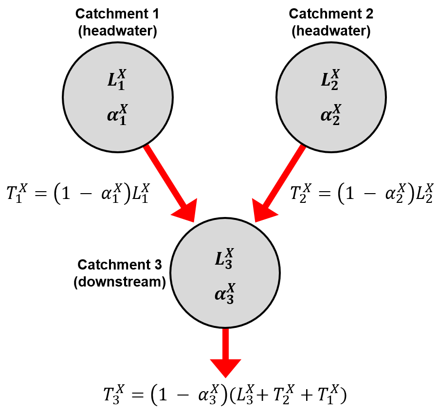
Fig. 1: Schematic illustration of the flux accumulation procedure in TEOTIL2. \(L_i^X\), sum of local inputs of parameter \(X\) to sub-catchment \(i\); \(\alpha_i^X\), retention factor for parameter \(X\) in sub-catchment \(i\); \(T_i^X\), load of \(X\) transmitted downstream from sub-catchment \(i\)